Analysing Climate Change and Temperature Anomalies

If we wanted to study climate change, we can find data on the Combined Land-Surface Air and Sea-Surface Water Temperature Anomalies in the Northern Hemisphere at NASA’s Goddard Institute for Space Studies. The tabular data of temperature anomalies can be found here

To define temperature anomalies you need to have a reference, or base, period which NASA clearly states that it is the period between 1951-1980.

Firstly, we need to load the file:

weather <- 
  read_csv("https://data.giss.nasa.gov/gistemp/tabledata_v3/NH.Ts+dSST.csv", 
           skip = 1, 
           na = "***")

Then we select the year and the months from the ‘weather’ dataset and convert it to a long format.

tidyweather <- weather %>%
  select(c(Year,Jan,Feb,Mar,Apr,May,Jun,Jul,Aug,Sep,Oct,Nov,Dec))%>%
  pivot_longer(cols = 2:13, names_to = "Month", values_to = "delta")
glimpse(tidyweather)

## Rows: 1,680
## Columns: 3
## $ Year  <dbl> 1880, 1880, 1880, 1880, 1880, 1880, 1880, 1880, 1880, 1880, 188…
## $ Month <chr> "Jan", "Feb", "Mar", "Apr", "May", "Jun", "Jul", "Aug", "Sep", …
## $ delta <dbl> -0.54, -0.38, -0.26, -0.37, -0.11, -0.22, -0.23, -0.24, -0.26, …

We observe that the dataframe has 3 variables: Year, Month, and Delta (Temperature Deviation)

Plotting Information

Let us plot the data using a time-series scatter plot, and add a trendline. To do that, we first need to create a new variable called date in order to ensure that the delta values are plot chronologically.

tidyweather <- tidyweather %>%
  mutate(date = ymd(paste(as.character(Year), Month, "1")),
         month = month(date, label=TRUE),
         year = year(date))
ggplot(tidyweather, aes(x=date, y = delta))+
  geom_point()+
  geom_smooth(color="red") +
  theme_bw() +
  labs (
    subtitle = "Weather Anomalies", 
    title = "Weather is becoming warmer and warmer"
  )+
  xlab("Date")+
  ylab("Temperature Deviation per month")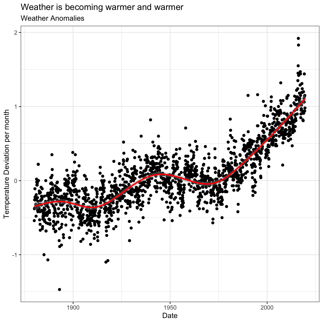

We create a scatter plot for each month.

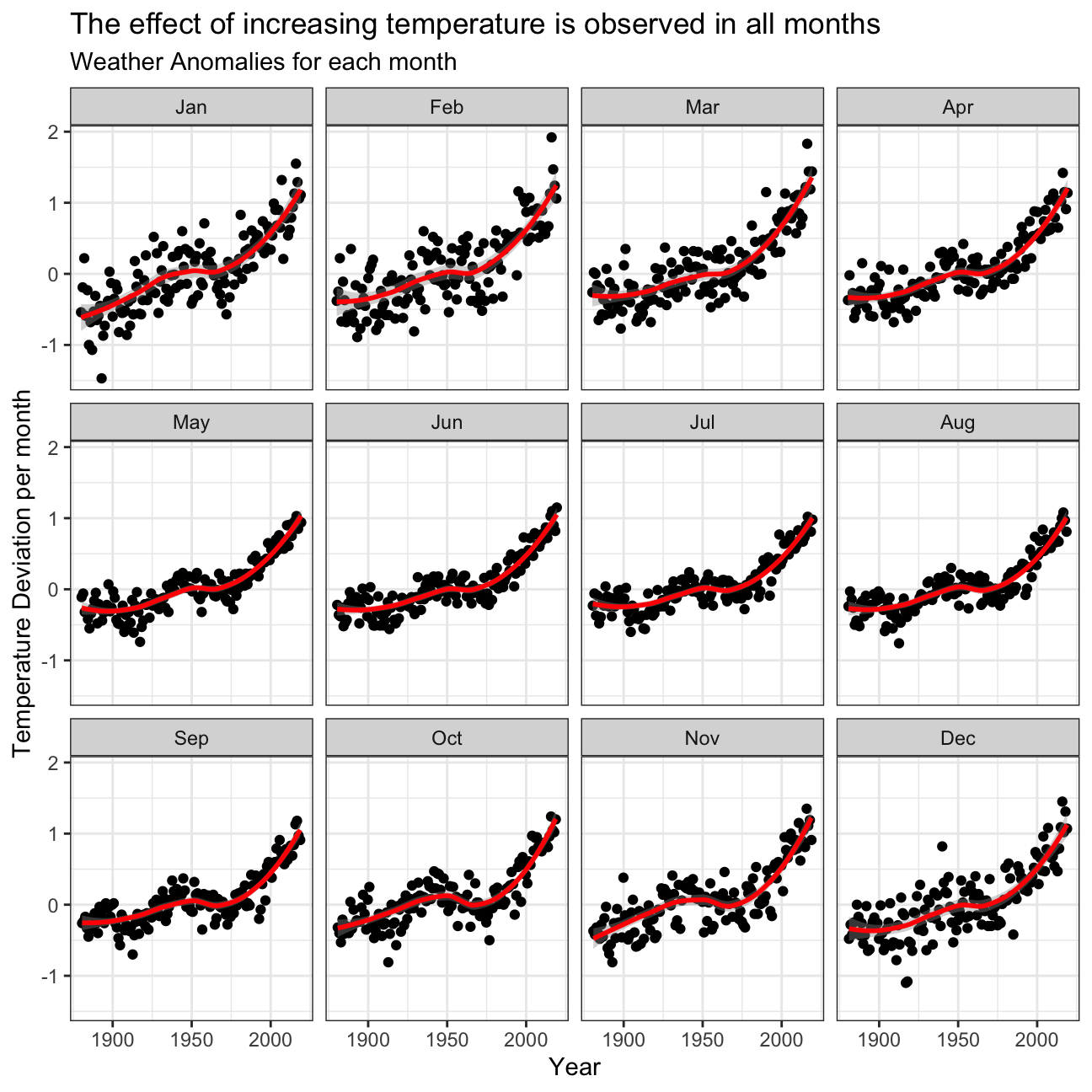
Looking at the plot we created, we observe that delta is increasing over time for all months. However, it seems that this increase is more pronounced in Winter. For instance, in October - March, the delta is closer to 1.5, whereas in the summer months it is around 1.

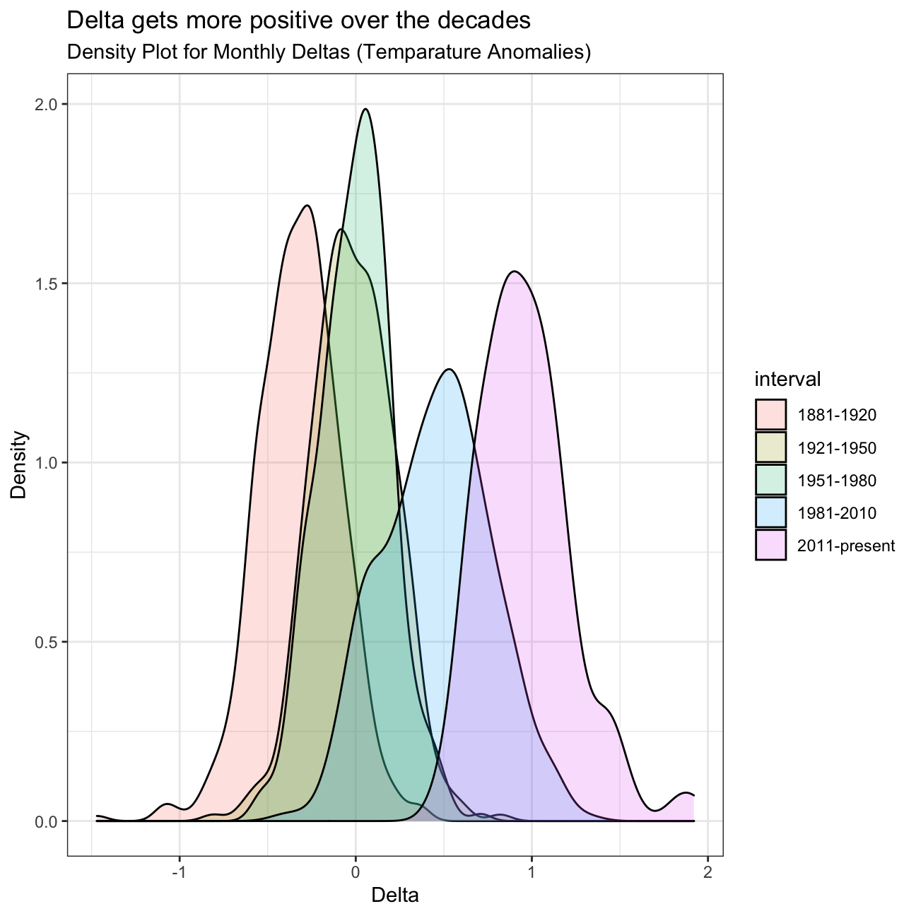
We would like to group the data into different time periods to study the large historical data. The most convenient way to do this is to refer to decades such as 1980s, 1990s etc. NASA calculates the temperature anomalies, as differed from the base period of 1951-1980. Thus, we create a new data frame called comparison that groups data in 5 time periods: 1881-1920, 1921-1950, 1951-1980, 1981-2010 and 2011-present.

We remove the data before 1800 and use mutate function to create a new variable intervals which contains information on which period each observation belongs to. We used case_when() to assign different periods.

comparison <- tidyweather %>% 
  filter(Year>= 1881) %>% 
  mutate(interval = case_when(
    Year %in% c(1881:1920) ~ "1881-1920",
    Year %in% c(1921:1950) ~ "1921-1950",
    Year %in% c(1951:1980) ~ "1951-1980",
    Year %in% c(1981:2010) ~ "1981-2010",
    TRUE ~ "2011-present"
  ))

Now that we have the interval variable, we can create a density plot to study the distribution of monthly deviations (delta), grouped by the different time periods we are interested in. Set fill to interval to group and colour the data by different time periods.

ggplot(comparison, aes(x=delta, fill=interval))+
  geom_density(alpha=0.2) + 
  theme_bw() +          
  labs (
    title = "Delta gets more positive over the decades",
    subtitle = "Density Plot for Monthly Deltas (Temparature Anomalies)",
    y     = "Density" ,
    x= "Delta"
  )

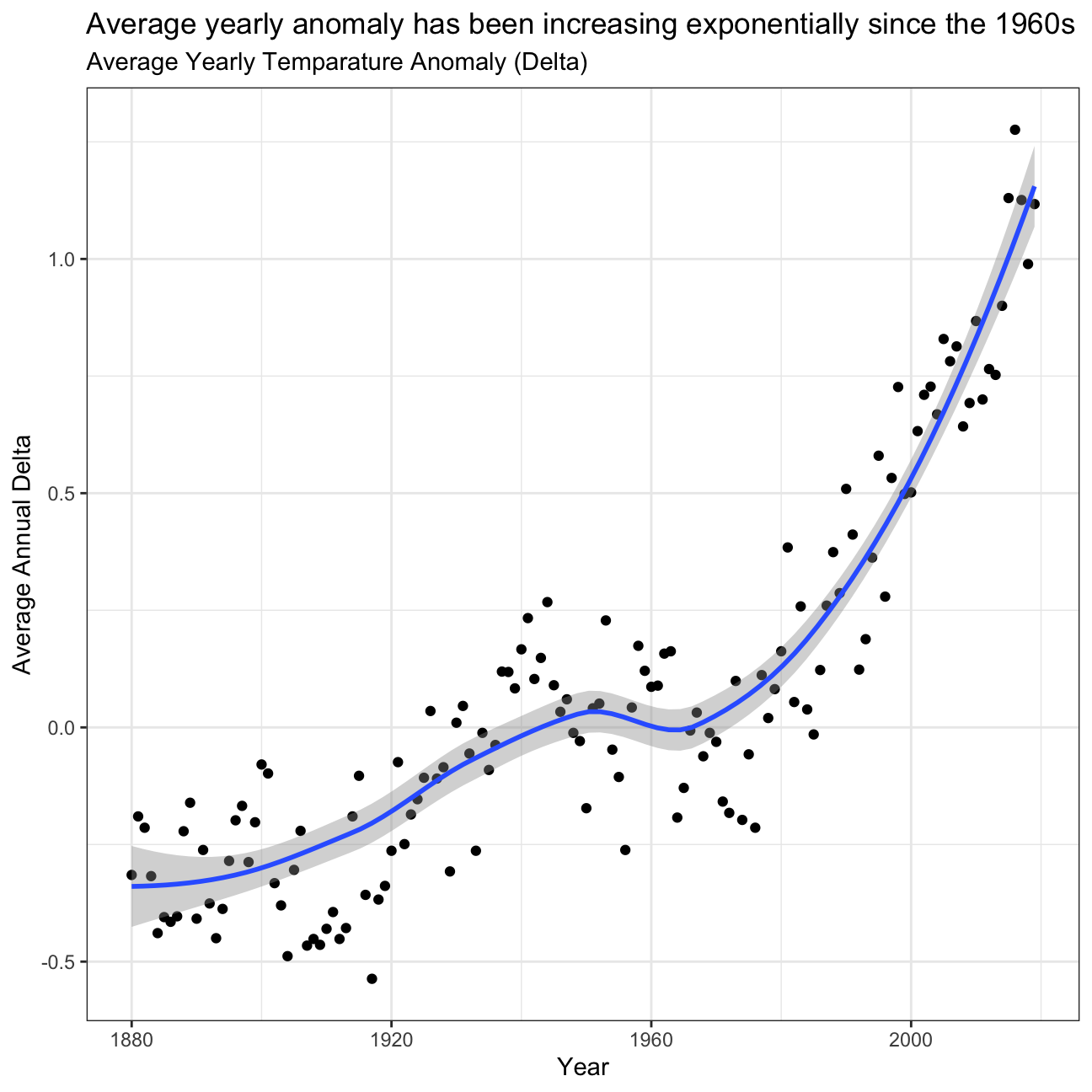
So far, we have been working with monthly anomalies. However, we might be interested in average annual anomalies. We can do this by using group_by() and summarise(), followed by a scatter plot to display the result.

avg_annual_anomaly <- tidyweather %>% 
  group_by(Year) %>%  
  # creating summaries for mean delta 
  summarise(annual_avg_delta = mean(delta, na.rm=TRUE)) 
ggplot(avg_annual_anomaly, aes(x=Year, y= annual_avg_delta))+
  geom_point()+
  geom_smooth() +
  theme_bw() +
  labs (
    title="Average yearly anomaly has been increasing exponentially since the 1960s",
    subtitle = "Average Yearly Temparature Anomaly (Delta)",
    y     = "Average Annual Delta"
  )                         

Confidence Interval for delta

NASA points out on their website that

A one-degree global change is significant because it takes a vast amount of heat to warm all the oceans, atmosphere, and land by that much. In the past, a one- to two-degree drop was all it took to plunge the Earth into the Little Ice Age. Now, we construct a 95% confidence interval for our data.

calculate_ci <- comparison %>% 
  filter(interval == "2011-present")%>%
  summarise(mean_diff=mean(delta,na.rm = TRUE),
            sd_diff=sd(delta, na.rm = TRUE), 
            count_diff=n(), 
            se_diff=sd_diff/sqrt(count_diff), 
            t_critical = qt(0.975, count_diff-1),
            lower = mean_diff-t_critical*se_diff,
            upper = mean_diff+t_critical*se_diff)
#print out formula_CI
calculate_ci

## # A tibble: 1 x 7
##   mean_diff sd_diff count_diff se_diff t_critical lower upper
##       <dbl>   <dbl>      <int>   <dbl>      <dbl> <dbl> <dbl>
## 1     0.966   0.262        108  0.0252       1.98 0.916  1.02

The 95% confidence interval for delta is 0.916-1.02.

Now, we use the bootstrap method to create a confidence interval.

# use the infer package to construct a 95% CI for delta
library(infer)
set.seed(1234)
data_infer <- comparison %>%
   filter(interval == "2011-present")%>%
  specify(response = delta)%>%
  generate(reps = 1000, type="bootstrap")%>%
  calculate(stat="mean")
percentile_ci <- data_infer %>%
  get_confidence_interval(level=0.95, type="percentile")
percentile_ci

## # A tibble: 1 x 2
##   lower_ci upper_ci
##      <dbl>    <dbl>
## 1    0.917     1.02

We have created two confidence intervals using two methods, one using our dataset and the other via bootstrapping for mean delta. The bootstrap method generates 1000 samples with replacement and approximates the distribution to estimate sample variability. The data shows us (for both methods, with the formula as well as with the infer package) that we can be 95% sure that the real mean of the population of temperature differences lies between 0.917 and 1.02.