How has it changed in years

# Import approval polls data
approval_polllist <- read_csv(here::here('data', 'approval_polllist.csv'))
# or directly off fivethirtyeight website
# approval_polllist <- read_csv('https://projects.fivethirtyeight.com/trump-approval-data/approval_polllist.csv') 
glimpse(approval_polllist)

## Rows: 14,533
## Columns: 22
## $ president           <chr> "Donald Trump", "Donald Trump", "Donald Trump", "…
## $ subgroup            <chr> "All polls", "All polls", "All polls", "All polls…
## $ modeldate           <chr> "8/29/2020", "8/29/2020", "8/29/2020", "8/29/2020…
## $ startdate           <chr> "1/20/2017", "1/20/2017", "1/20/2017", "1/21/2017…
## $ enddate             <chr> "1/22/2017", "1/22/2017", "1/24/2017", "1/23/2017…
## $ pollster            <chr> "Gallup", "Morning Consult", "Ipsos", "Gallup", "…
## $ grade               <chr> "B", "B/C", "B-", "B", "B", "C+", "B-", "B+", "B"…
## $ samplesize          <dbl> 1500, 1992, 1632, 1500, 1500, 1500, 1651, 1190, 2…
## $ population          <chr> "a", "rv", "a", "a", "a", "lv", "a", "rv", "a", "…
## $ weight              <dbl> 0.262, 0.680, 0.153, 0.243, 0.227, 0.200, 0.142, …
## $ influence           <dbl> 0, 0, 0, 0, 0, 0, 0, 0, 0, 0, 0, 0, 0, 0, 0, 0, 0…
## $ approve             <dbl> 45.0, 46.0, 42.1, 45.0, 46.0, 57.0, 42.3, 36.0, 4…
## $ disapprove          <dbl> 45.0, 37.0, 45.2, 46.0, 45.0, 43.0, 45.8, 44.0, 3…
## $ adjusted_approve    <dbl> 45.8, 45.3, 43.2, 45.8, 46.8, 51.6, 43.4, 37.7, 4…
## $ adjusted_disapprove <dbl> 43.6, 37.8, 43.9, 44.6, 43.6, 44.4, 44.5, 42.8, 3…
## $ multiversions       <chr> NA, NA, NA, NA, NA, NA, NA, NA, NA, NA, NA, NA, N…
## $ tracking            <lgl> TRUE, NA, TRUE, TRUE, TRUE, TRUE, TRUE, NA, NA, T…
## $ url                 <chr> "http://www.gallup.com/poll/201617/gallup-daily-t…
## $ poll_id             <dbl> 49253, 49249, 49426, 49262, 49236, 49266, 49425, …
## $ question_id         <dbl> 77265, 77261, 77599, 77274, 77248, 77278, 77598, …
## $ createddate         <chr> "1/23/2017", "1/23/2017", "3/1/2017", "1/24/2017"…
## $ timestamp           <chr> "13:38:37 29 Aug 2020", "13:38:37 29 Aug 2020", "…

# Use `lubridate` to fix dates, as they are given as characters.

Create a plot

We calculate the average net approval rate (approve- disapprove) for each week since he got into office. We plot the net approval, along with its 95% confidence interval.

approval_polllist <- approval_polllist %>% 
  mutate(net_approval = approve - disapprove,
         date = mdy(enddate),
         year = year(date),
         week = week(date))
Trump_approval_margin <- approval_polllist %>% 
  group_by(year, week) %>% 
  summarise(mean_net_approval = mean(net_approval),
            sd_net_approval = sd(net_approval),
            count = n(),
            t_critical = qt(0.975, count-1),
            se_net_approval = sd_net_approval/sqrt(count),
            low_net_approval = mean_net_approval - t_critical*se_net_approval,
            high_net_approval = mean_net_approval + t_critical*se_net_approval)

Trump_plot <- Trump_approval_margin %>% 
  ggplot(aes(x = week, y = mean_net_approval, color = as.factor(year))) +
  geom_ribbon(aes(ymin = low_net_approval, ymax = high_net_approval, fill = as.factor(year))) +
  geom_line() +
  geom_point() +
  facet_wrap(~year) +
  scale_color_manual(values = c("#FF0000", "#32CD32", "#236B81", "#9932CD", "organge")) +
  scale_fill_manual(values = alpha(c("#FF0000", "#32CD32", "#236B81", "#9932CD"), 0.1)) +
  scale_x_continuous(breaks = c(0, 13, 26, 39, 52)) +
  scale_y_continuous(breaks = seq(-20, 7.5, by = 2.5)) +
  coord_fixed(ratio = 1/1.5) +
  geom_hline(aes(yintercept=0), color = "orange") +
  labs(title = "The average approval for Trump started to get volatile again recently", 
       subtitle = "Estimating Net Approval (approve-disapprove) for Donald Trump (Weekly average of all polls)",
       x = "Week of the year",
       y = "Average Net Approval (%)") +
  theme(legend.position = "none") +
  theme_bw()
Trump_plot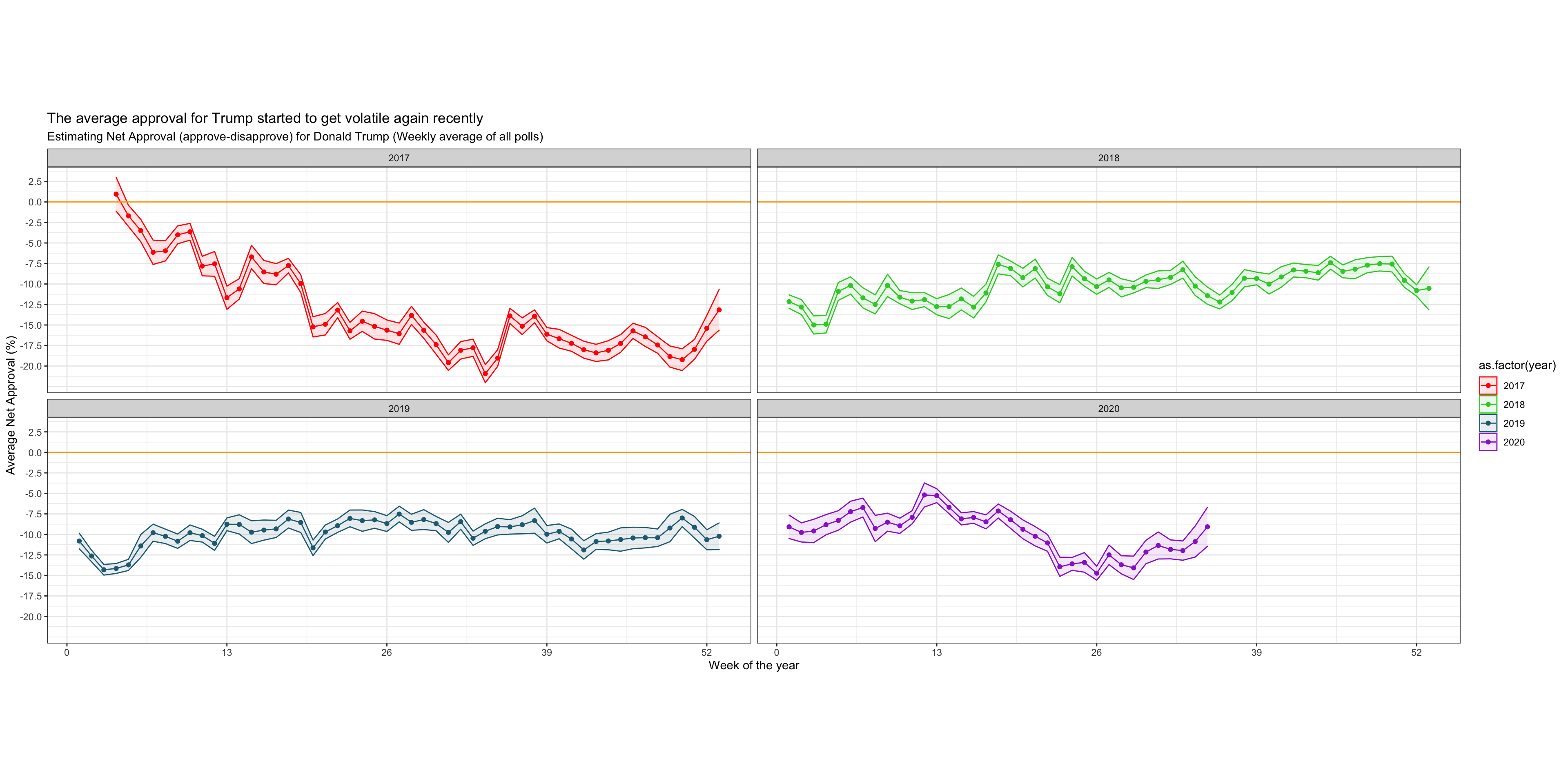

We facet by year, and add an orange line at zero.

Compare Confidence Intervals for week 15 and week 34 in 2020

We compare the confidence intervals for ‘week 15’ (6-12 April 2020) and ‘week 34’ (17-23 August 2020).

Trump_approval_margin %>% 
  filter(week %in% c(15, 34), year == 2020) %>% 
  select(c(year, week, low_net_approval, high_net_approval))

## # A tibble: 2 x 4
## # Groups:   year [1]
##    year  week low_net_approval high_net_approval
##   <dbl> <dbl>            <dbl>             <dbl>
## 1  2020    15            -8.84             -7.36
## 2  2020    34           -12.8              -8.98

Based on the results above, in week 34 confidence interval is longer due to a higher standard error which can be due to t-critical value or standard deviation. In both, week 15 and week 34 t-critical values are approximately the same, therefore standard distribution in week 34 is higher indicating poor results. It is then difficult to predict true mean. The reason of this fall might be Trump’s attitude during the beginning of the Coronavirus outbreak.